KGTopologyToolbox walk-through
Copyright (c) 2024 Graphcore Ltd. All rights reserved.
In this notebook we give a general overview of the classes and methods included in the kg-topology-toolbox library and explain how to use them to extract topological data from any knowledge graph. As an example, we use the open-source biomedical dataset ogbl-biokg.
Dependencies
[1]:
import sys
!{sys.executable} -m pip uninstall -y kg_topology_toolbox
!pip install -q git+https://github.com/graphcore-research/kg-topology-toolbox.git --no-cache-dir
!pip install -q jupyter ipywidgets ogb seaborn
Found existing installation: kg-topology-toolbox 1.0.0
Uninstalling kg-topology-toolbox-1.0.0:
  Successfully uninstalled kg-topology-toolbox-1.0.0
[1]:
import numpy as np
import pandas as pd
import matplotlib.pyplot as plt
import seaborn as sns

import ogb.linkproppred
from kg_topology_toolbox import KGTopologyToolbox

dataset_directory = "../../../data/ogb-biokg/"
Data preparation
We load the OGBL-BioKG dataset using the ogb.linkproppred.LinkPropPredDataset class and store all (h, r, t) triples in a pandas DataFrame.
[2]:
dataset = ogb.linkproppred.LinkPropPredDataset(
    name="ogbl-biokg", root=dataset_directory
)

all_triples = []
for split in dataset.get_edge_split().values():
    all_triples.append(np.stack([split["head"], split["relation"], split["tail"]]).T)
biokg_df = pd.DataFrame(
    np.concatenate(all_triples).astype(np.int32), columns=["h", "r", "t"]
)
biokg_df
[2]:
| h | r | t | |
|---|---|---|---|
| 0 | 1718 | 0 | 3207 |
| 1 | 4903 | 0 | 13662 |
| 2 | 5480 | 0 | 15999 |
| 3 | 3148 | 0 | 7247 |
| 4 | 10300 | 0 | 16202 |
| ... | ... | ... | ... |
| 5088429 | 2451 | 50 | 5097 |
| 5088430 | 6456 | 50 | 8833 |
| 5088431 | 9484 | 50 | 15873 |
| 5088432 | 6365 | 50 | 496 |
| 5088433 | 13860 | 50 | 6368 |
5088434 rows × 3 columns
Based on this representation of the knowledge graph, we can proceed to instantiate the KGTopologyToolbox class to compute topological properties.
[6]:
kgtt = KGTopologyToolbox(biokg_df)
/nethome/albertoc/research/knowledge_graphs/kg-topology-toolbox/.venv/lib/python3.10/site-packages/kg_topology_toolbox/utils.py:42: UserWarning: The Knowledge Graph contains duplicated edges -- some functionalities may produce incorrect results
  warnings.warn(
Notice the warning raised by the constructor, which detects duplicated edges in the biokg_df DataFrame: to ensure optimal functionalities, duplicated edges should be removed before instantiating the KGTopologyToolbox class.
[8]:
# find duplicated edges
biokg_df.loc[biokg_df.duplicated(keep=False)]
[8]:
| h | r | t | |
|---|---|---|---|
| 3854407 | 1972 | 45 | 1972 |
| 4000534 | 1972 | 45 | 1972 |
Node-level analysis
The method node_degree_summary provides a summary of the degrees of each individual node in the knowledge graph. The returned DataFrame is indexed on the node ID.
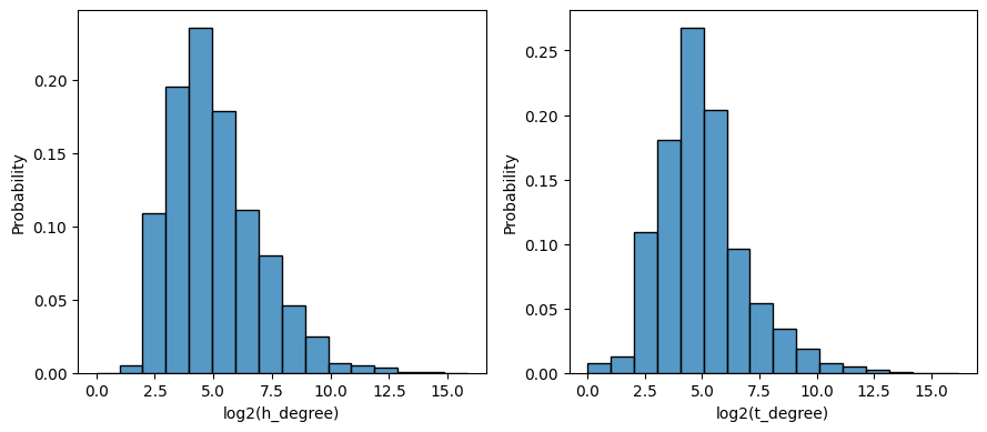
h_degreeis the number of edges coming out from the node;t_degreeis the number of edges going into the node;tot_degreeis the number of edges that use the node as either head or tail;h_unique_rel(resp.,t_unique_rel) is the number of unique relation types that come out from (resp., go into) the node;n_loopsis the number of loop edges around the node.
[5]:
node_ds = kgtt.node_degree_summary()
node_ds
[5]:
| h_degree | t_degree | tot_degree | h_unique_rel | t_unique_rel | n_loops | |
|---|---|---|---|---|---|---|
| 0 | 27 | 72 | 99 | 4 | 4 | 0 |
| 1 | 14 | 94 | 108 | 3 | 6 | 0 |
| 2 | 208 | 95 | 303 | 5 | 7 | 0 |
| 3 | 28999 | 26154 | 55153 | 10 | 11 | 0 |
| 4 | 362 | 302 | 664 | 11 | 12 | 0 |
| ... | ... | ... | ... | ... | ... | ... |
| 45080 | 21 | 22 | 43 | 1 | 1 | 0 |
| 45081 | 29 | 32 | 61 | 1 | 1 | 0 |
| 45082 | 28 | 30 | 58 | 1 | 1 | 0 |
| 45083 | 17 | 19 | 36 | 1 | 1 | 0 |
| 45084 | 28 | 31 | 59 | 1 | 1 | 0 |
45085 rows × 6 columns
[6]:
metrics = [
    "h_degree",
    "t_degree",
]
fig, ax = plt.subplots(1, len(metrics), figsize=(4.5 * len(metrics), 4))

for i, metric in enumerate(metrics):
    x = np.log2(node_ds[metric])
    sns.histplot(
        x=x, stat="probability", binwidth=1, binrange=[0, x.max() + 1], ax=ax[i]
    )
    ax[i].set_xlabel(f"log2({metric})")
plt.tight_layout()
/nethome/albertoc/research/knowledge_graphs/kg-topology-toolbox/.venv/lib/python3.10/site-packages/pandas/core/arraylike.py:399: RuntimeWarning: divide by zero encountered in log2
  result = getattr(ufunc, method)(*inputs, **kwargs)
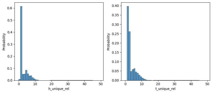
[7]:
metrics = [
    "h_unique_rel",
    "t_unique_rel",
]
fig, ax = plt.subplots(1, len(metrics), figsize=(4.5 * len(metrics), 4))

for i, metric in enumerate(metrics):
    x = node_ds[metric]
    sns.histplot(
        x=x, stat="probability", binwidth=1, binrange=[0, x.max() + 1], ax=ax[i]
    )
    ax[i].set_xlabel(f"{metric}")
plt.tight_layout()
Edge-level analysis
Edge degrees and cardinality
The method edge_degree_cardinality_summary provides, for each edge (h, r, t) in the KG, detailed information on the connectivity patterns of the head and tail nodes:
h_unique_rel(resp.t_unique_rel) is the number of unique relation types coming out of the head node (resp. going into the tail node);h_degreeis the out-degree of the head node andh_degree_same_relis the degree when only considering edges of the same relation typer;t_degreeis the in-degree of the tail node andt_degree_same_relis the degree when only considering edges of the same relation typer;tot_degreeis the total number of edges with either head entityhor tail entityt(in particular,tot_degree <= h_degree + t_degree);tot_degree_same_relis computed only considering edges of the same relation typer;triple_cardinalityis the cardinality type of the edge:one-to-one (1:1) if
h_degree = 1,t_degree = 1;one-to-many (1:M) if
h_degree > 1,t_degree = 1;many-to-one (M:1) if
h_degree = 1,t_degree > 1;many-to-many (M:M) if
h_degree > 1,t_degree > 1.
triple_cardinality_same_relis defined astriple_cardinalitybut usingh_degree_same_rel,t_degree_same_rel.
[8]:
edge_dcs = kgtt.edge_degree_cardinality_summary()
edge_dcs
[8]:
| h | r | t | h_degree | h_unique_rel | h_degree_same_rel | t_degree | t_unique_rel | t_degree_same_rel | tot_degree | tot_degree_same_rel | triple_cardinality | triple_cardinality_same_rel | |
|---|---|---|---|---|---|---|---|---|---|---|---|---|---|
| 0 | 1718 | 0 | 3207 | 191 | 5 | 116 | 46 | 6 | 14 | 236 | 129 | M:M | M:M |
| 1 | 4903 | 0 | 13662 | 544 | 8 | 33 | 1975 | 9 | 50 | 2518 | 82 | M:M | M:M |
| 2 | 5480 | 0 | 15999 | 108 | 3 | 5 | 72 | 4 | 22 | 179 | 26 | M:M | M:M |
| 3 | 3148 | 0 | 7247 | 110 | 4 | 99 | 673 | 11 | 271 | 782 | 369 | M:M | M:M |
| 4 | 10300 | 0 | 16202 | 414 | 4 | 315 | 148 | 6 | 31 | 561 | 345 | M:M | M:M |
| ... | ... | ... | ... | ... | ... | ... | ... | ... | ... | ... | ... | ... | ... |
| 5088429 | 2451 | 50 | 5097 | 636 | 5 | 272 | 803 | 10 | 272 | 1437 | 543 | M:M | M:M |
| 5088430 | 6456 | 50 | 8833 | 743 | 10 | 259 | 371 | 10 | 100 | 1111 | 358 | M:M | M:M |
| 5088431 | 9484 | 50 | 15873 | 652 | 8 | 213 | 486 | 6 | 163 | 1135 | 375 | M:M | M:M |
| 5088432 | 6365 | 50 | 496 | 922 | 9 | 277 | 618 | 19 | 173 | 1537 | 449 | M:M | M:M |
| 5088433 | 13860 | 50 | 6368 | 485 | 7 | 175 | 455 | 8 | 147 | 939 | 321 | M:M | M:M |
5088434 rows × 13 columns
The data on the distribution of degrees and cardinalities can be then easily visualized.
[9]:
# Edge frequency when binning by head and tail degree

metrics = [("h_degree", "t_degree"), ("h_degree_same_rel", "t_degree_same_rel")]
fig, ax = plt.subplots(1, len(metrics), figsize=[5 * len(metrics), 4.5])

for i, (group_metric_1, group_metric_2) in enumerate(metrics):
    df_empty = pd.DataFrame(
        columns=np.int32(2 ** np.arange(15)), index=np.int32(2 ** np.arange(15))
    )
    df_tmp = edge_dcs[[group_metric_1, group_metric_2]]
    df_tmp.insert(
        0,
        f"log_{group_metric_1}",
        np.int32(2 ** np.floor(np.log2(df_tmp[group_metric_1]))),
    )
    df_tmp.insert(
        0,
        f"log_{group_metric_2}",
        np.int32(2 ** np.floor(np.log2(df_tmp[group_metric_2]))),
    )
    df_tmp = (
        df_tmp.groupby([f"log_{group_metric_1}", f"log_{group_metric_2}"])
        .count()
        .reset_index()
    )
    df_tmp[group_metric_1] /= df_tmp[group_metric_1].sum()
    sns.heatmap(
        df_tmp.reset_index()
        .pivot(
            columns=f"log_{group_metric_2}",
            index=f"log_{group_metric_1}",
            values=group_metric_1,
        )
        .combine_first(df_empty),
        annot=False,
        vmin=0,
        vmax=0.05,
        ax=ax[i],
    )
    ax[i].set_xlabel(group_metric_2)
    ax[i].set_ylabel(group_metric_1)
    ax[i].invert_yaxis()
fig.suptitle("Edge frequency")
plt.tight_layout()
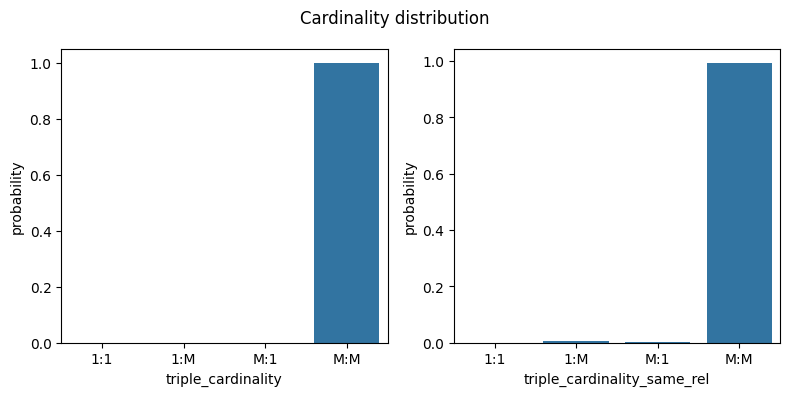
[10]:
metrics = ["triple_cardinality", "triple_cardinality_same_rel"]
fig, ax = plt.subplots(1, len(metrics), figsize=[4 * len(metrics), 4])

for i, metric in enumerate(metrics):
    sns.countplot(
        x=edge_dcs[metric],
        order=["1:1", "1:M", "M:1", "M:M"],
        stat="probability",
        ax=ax[i],
    )
fig.suptitle("Cardinality distribution")
plt.tight_layout()

Edge topological patterns
KGTopologyToolbox also allows us to perform a topological analysis at the edge level, using the method edge_pattern_summary, which extracts information on several significant edge topological patterns. In particular, it detects whether the edge (h,r,t) is a loop, is symmetric or has inverse, inference, composition (directed and undirected):
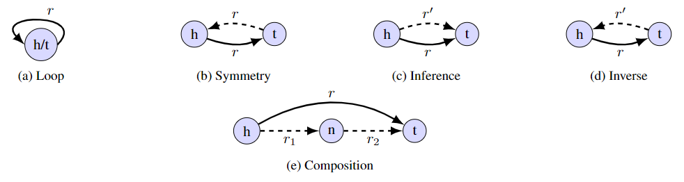
For inverse/inference, the method also provides the number and types of unique relations r' realizing the counterpart edges; for composition, the number of triangles supported by the edge is provided.
[11]:
edge_eps = kgtt.edge_pattern_summary()
edge_eps
[11]:
| h | r | t | is_loop | is_symmetric | has_inverse | n_inverse_relations | inverse_edge_types | has_inference | n_inference_relations | inference_edge_types | has_composition | has_undirected_composition | n_triangles | n_undirected_triangles | |
|---|---|---|---|---|---|---|---|---|---|---|---|---|---|---|---|
| 0 | 1718 | 0 | 3207 | False | False | False | 0 | [] | False | 0 | [0] | False | True | 0 | 15 |
| 1 | 4903 | 0 | 13662 | False | False | False | 0 | [] | False | 0 | [0] | True | True | 44 | 153 |
| 2 | 5480 | 0 | 15999 | False | False | False | 0 | [] | False | 0 | [0] | False | True | 0 | 1 |
| 3 | 3148 | 0 | 7247 | False | False | False | 0 | [] | False | 0 | [0] | True | True | 10 | 29 |
| 4 | 10300 | 0 | 16202 | False | False | False | 0 | [] | False | 0 | [0] | True | True | 3 | 79 |
| ... | ... | ... | ... | ... | ... | ... | ... | ... | ... | ... | ... | ... | ... | ... | ... |
| 5088429 | 2451 | 50 | 5097 | False | False | True | 1 | [46] | True | 1 | [46, 50] | True | True | 1532 | 5722 |
| 5088430 | 6456 | 50 | 8833 | False | False | True | 2 | [45, 46] | True | 2 | [45, 46, 50] | True | True | 234 | 913 |
| 5088431 | 9484 | 50 | 15873 | False | False | True | 1 | [46] | True | 2 | [46, 45, 50] | True | True | 1326 | 5004 |
| 5088432 | 6365 | 50 | 496 | False | False | True | 2 | [45, 46] | True | 2 | [45, 46, 50] | True | True | 1433 | 5554 |
| 5088433 | 13860 | 50 | 6368 | False | False | False | 0 | [] | False | 0 | [50] | True | True | 119 | 489 |
5088434 rows × 15 columns
If we need to identify the different metapaths [r_1, r_2] that give triangles (h,r1,x) - (x,r2,t) over an edge (h,r,t), we can do so by setting return_metapath_list=True in the call of edge_pattern_summary. In order to disaggregate the total number of triangles over an edge into separate counts for each existing metapath, the edge_metapath_count method should be used instead.
We can now easily produce a global view of the distribution of topological properties.
[12]:
print("Fraction of triples with property:")
edge_eps[
    ["is_loop", "is_symmetric", "has_inverse", "has_inference", "has_composition"]
].mean()
Fraction of triples with property:
[12]:
is_loop            0.000011
is_symmetric       0.713743
has_inverse        0.409704
has_inference      0.410111
has_composition    0.997605
dtype: float64
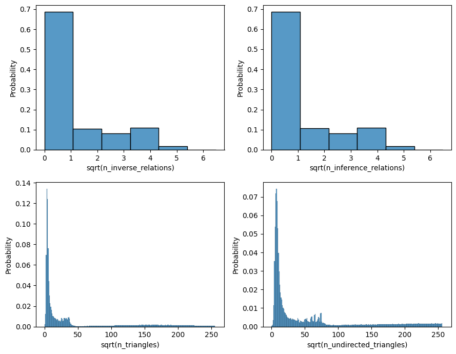
[13]:
metrics = [
    "n_inverse_relations",
    "n_inference_relations",
    "n_triangles",
    "n_undirected_triangles",
]
fig, ax = plt.subplots(2, 2, figsize=(9, 7))

for axn, metric in zip(ax.flatten(), metrics):
    x = np.sqrt(edge_eps[metric])
    sns.histplot(x=x, stat="probability", binwidth=1, binrange=[0, x.max() + 1], ax=axn)
    axn.set_xlabel(f"sqrt({metric})")
plt.tight_layout()
Filtering relation types
The edge-level methods presented in the previous section simultaneously compute statistics for all edges in the KG, and this can be expensive on larger graphs. Moreover, in many practical cases the user might be interested in looking only at the properties of edges of one or few specific relation types.
The methods edge_degree_cardinality_summary, edge_pattern_summary and edge_metapath_count can be passed a list of relation type IDs to restrict computations of their outputs to edges of those specific relation types.
[7]:
filtered_metapath_counts = kgtt.edge_metapath_count(filter_relations=[7, 24])
filtered_metapath_counts
[7]:
| index | h | r | t | r1 | r2 | n_triangles | |
|---|---|---|---|---|---|---|---|
| 0 | 334382 | 732 | 7 | 1225 | 41 | 2 | 10 |
| 1 | 334382 | 732 | 7 | 1225 | 39 | 2 | 123 |
| 2 | 334382 | 732 | 7 | 1225 | 38 | 2 | 200 |
| 3 | 334382 | 732 | 7 | 1225 | 37 | 2 | 27 |
| 4 | 334382 | 732 | 7 | 1225 | 36 | 2 | 6 |
| ... | ... | ... | ... | ... | ... | ... | ... |
| 732149 | 4953327 | 1529 | 24 | 2492 | 13 | 41 | 2 |
| 732150 | 4953327 | 1529 | 24 | 2492 | 11 | 41 | 2 |
| 732151 | 4953327 | 1529 | 24 | 2492 | 6 | 41 | 2 |
| 732152 | 4953327 | 1529 | 24 | 2492 | 4 | 41 | 1 |
| 732153 | 4953327 | 1529 | 24 | 2492 | 2 | 41 | 2 |
732154 rows × 7 columns
The previous cell computes the number of triangles of each existing (r1, r2) metapath, but only over (h,r,t) edges of the two relation types with ID 7 and 24 (the column index gives the index of the edge in the biokkg_df DataFrame). This is the same as calling kgtt.edge_metapath_count().query('r==7 or r==24'), but the computation is much cheaper and faster.
[8]:
filtered_metapath_counts.r.value_counts()
[8]:
r
24    413366
7     318788
Name: count, dtype: int64
Relation-level analysis
All edge topological properties seen in the previous section can be aggregated over triples of the same relation type, to produce relation-level statistics. To do so, we can either set the option aggregate_by_r = True when calling the methods edge_degree_cardinality_summary, edge_pattern_summary, or - if edge topological metrics have already been precomputed - use the utility function aggregate_by_relation, which converts DataFrames indexed on the KG edges to DataFrames indexed
on the IDs of the unique relation types.
[15]:
from kg_topology_toolbox.utils import aggregate_by_relation

aggregate_by_relation(edge_dcs).head()
[15]:
| num_triples | frac_triples | unique_h | unique_t | h_degree_mean | h_degree_std | h_degree_quartile1 | h_degree_quartile2 | h_degree_quartile3 | h_unique_rel_mean | ... | tot_degree_same_rel_quartile1 | tot_degree_same_rel_quartile2 | tot_degree_same_rel_quartile3 | triple_cardinality_1:M_frac | triple_cardinality_M:1_frac | triple_cardinality_M:M_frac | triple_cardinality_same_rel_1:1_frac | triple_cardinality_same_rel_1:M_frac | triple_cardinality_same_rel_M:1_frac | triple_cardinality_same_rel_M:M_frac | |
|---|---|---|---|---|---|---|---|---|---|---|---|---|---|---|---|---|---|---|---|---|---|
| r | |||||||||||||||||||||
| 0 | 81066 | 0.015931 | 9742 | 9337 | 569.252202 | 1083.315332 | 111.0 | 222.0 | 521.0 | 8.110293 | ... | 45.0 | 112.0 | 211.0 | 0.0 | 0.0 | 1.0 | 0.001628 | 0.023586 | 0.064959 | 0.909827 |
| 1 | 5669 | 0.001114 | 698 | 1536 | 2518.765391 | 2186.452620 | 435.0 | 2087.0 | 4028.0 | 27.048157 | ... | 14.0 | 32.0 | 60.0 | 0.0 | 0.0 | 1.0 | 0.002822 | 0.104251 | 0.027518 | 0.865408 |
| 2 | 66954 | 0.013158 | 612 | 612 | 4129.511919 | 1935.630599 | 2548.0 | 3968.0 | 5649.0 | 36.404307 | ... | 332.0 | 404.0 | 482.0 | 0.0 | 0.0 | 1.0 | 0.000000 | 0.000254 | 0.000239 | 0.999507 |
| 3 | 19585 | 0.003849 | 491 | 491 | 4527.399592 | 1943.714179 | 2925.0 | 4507.0 | 6161.0 | 37.095941 | ... | 114.0 | 157.0 | 202.0 | 0.0 | 0.0 | 1.0 | 0.000000 | 0.000868 | 0.000970 | 0.998162 |
| 4 | 32034 | 0.006295 | 526 | 525 | 4511.067834 | 1905.395180 | 2931.0 | 4507.0 | 6148.0 | 37.319567 | ... | 188.0 | 243.0 | 299.0 | 0.0 | 0.0 | 1.0 | 0.000062 | 0.000531 | 0.000593 | 0.998814 |
5 rows × 51 columns
Notice on the extra columns num_triples, frac_triples, unique_h, unique_t giving additional statistics for relation types (number of edges and relative frequency, number of unique entities used as heads/tails by triples of the relation type).
Similarly, by aggregating the edge_eps DataFrame we can look at the distribution of edge topological patterns within each relation type.
[16]:
aggregate_by_relation(edge_eps).head()
[16]:
| num_triples | frac_triples | unique_h | unique_t | is_loop_frac | is_symmetric_frac | has_inverse_frac | n_inverse_relations_mean | n_inverse_relations_std | n_inverse_relations_quartile1 | ... | n_triangles_mean | n_triangles_std | n_triangles_quartile1 | n_triangles_quartile2 | n_triangles_quartile3 | n_undirected_triangles_mean | n_undirected_triangles_std | n_undirected_triangles_quartile1 | n_undirected_triangles_quartile2 | n_undirected_triangles_quartile3 | |
|---|---|---|---|---|---|---|---|---|---|---|---|---|---|---|---|---|---|---|---|---|---|
| r | |||||||||||||||||||||
| 0 | 81066 | 0.015931 | 9742 | 9337 | 0.000012 | 0.000222 | 0.009474 | 0.018762 | 0.336120 | 0.0 | ... | 49.615572 | 816.776738 | 3.0 | 7.0 | 16.00 | 136.452841 | 1421.830008 | 18.00 | 36.0 | 68.0 |
| 1 | 5669 | 0.001114 | 698 | 1536 | 0.000000 | 0.000353 | 0.061563 | 0.527783 | 2.502323 | 0.0 | ... | 1630.912154 | 6563.522736 | 13.0 | 84.0 | 234.00 | 2864.104428 | 9520.116812 | 54.00 | 224.0 | 586.0 |
| 2 | 66954 | 0.013158 | 612 | 612 | 0.000000 | 0.947367 | 0.998253 | 11.019118 | 4.707246 | 8.0 | ... | 27666.694925 | 15797.649746 | 14990.0 | 25934.0 | 38868.50 | 32678.993563 | 18619.016056 | 16691.00 | 32647.5 | 48637.0 |
| 3 | 19585 | 0.003849 | 491 | 491 | 0.000000 | 0.947358 | 0.999592 | 13.417258 | 4.585150 | 10.0 | ... | 30250.858974 | 17053.925410 | 16204.0 | 28873.0 | 43798.00 | 32696.125351 | 18685.281686 | 16563.00 | 32808.0 | 48653.0 |
| 4 | 32034 | 0.006295 | 526 | 525 | 0.000000 | 0.947368 | 0.999376 | 13.299588 | 4.427898 | 10.0 | ... | 30942.231192 | 16888.956656 | 17303.0 | 30137.5 | 44161.25 | 32685.210464 | 18685.267154 | 16645.25 | 32580.0 | 48767.0 |
5 rows × 32 columns
Additional methods are provided in the KGTopologyToolbox class for analysis at the relation level: jaccard_similarity_relation_sets to compute the Jaccard similarity of the sets of head/tail entities used by each relation; relational_affinity_ingram to compute the InGram pairwise relation similarity (see paper).
[17]:
kgtt.jaccard_similarity_relation_sets()
[17]:
| r1 | r2 | num_triples_both | frac_triples_both | num_entities_both | num_h_r1 | num_h_r2 | num_t_r1 | num_t_r2 | jaccard_head_head | jaccard_head_tail | jaccard_tail_head | jaccard_tail_tail | jaccard_both | |
|---|---|---|---|---|---|---|---|---|---|---|---|---|---|---|
| 1 | 0 | 1 | 86735 | 0.017046 | 14338 | 9742 | 698 | 9337 | 1536 | 0.064112 | 0.055301 | 0.037317 | 0.079635 | 0.112289 |
| 2 | 0 | 2 | 148020 | 0.029089 | 13934 | 9742 | 612 | 9337 | 612 | 0.056531 | 0.056531 | 0.031947 | 0.031947 | 0.041768 |
| 3 | 0 | 3 | 100651 | 0.019780 | 13929 | 9742 | 491 | 9337 | 491 | 0.045037 | 0.045037 | 0.026530 | 0.026530 | 0.033527 |
| 4 | 0 | 4 | 113100 | 0.022227 | 13931 | 9742 | 526 | 9337 | 525 | 0.048290 | 0.048188 | 0.027610 | 0.027506 | 0.035819 |
| 5 | 0 | 5 | 132276 | 0.025995 | 13931 | 9742 | 576 | 9337 | 578 | 0.053287 | 0.053491 | 0.029815 | 0.029916 | 0.039624 |
| ... | ... | ... | ... | ... | ... | ... | ... | ... | ... | ... | ... | ... | ... | ... |
| 2446 | 47 | 49 | 18021 | 0.003542 | 2414 | 806 | 1885 | 809 | 1886 | 0.131148 | 0.131568 | 0.132409 | 0.132353 | 0.135874 |
| 2447 | 47 | 50 | 374193 | 0.073538 | 5592 | 806 | 5224 | 809 | 5228 | 0.082391 | 0.082526 | 0.083318 | 0.083453 | 0.084764 |
| 2497 | 48 | 49 | 43122 | 0.008475 | 3407 | 2728 | 1885 | 2729 | 1886 | 0.371284 | 0.369952 | 0.371989 | 0.371064 | 0.370707 |
| 2498 | 48 | 50 | 399294 | 0.078471 | 6201 | 2728 | 5224 | 2729 | 5228 | 0.287356 | 0.287379 | 0.286061 | 0.286084 | 0.289147 |
| 2549 | 49 | 50 | 388092 | 0.076269 | 6169 | 1885 | 5224 | 1886 | 5228 | 0.156876 | 0.156773 | 0.156850 | 0.156748 | 0.158373 |
1275 rows × 14 columns
[18]:
kgtt.relational_affinity_ingram()
[18]:
| h_relation | t_relation | edge_weight | |
|---|---|---|---|
| 0 | 0 | 1 | 5.565931 |
| 1 | 0 | 2 | 0.244410 |
| 2 | 0 | 3 | 0.049564 |
| 3 | 0 | 4 | 0.079068 |
| 4 | 0 | 5 | 0.159787 |
| ... | ... | ... | ... |
| 2545 | 50 | 45 | 393.082900 |
| 2546 | 50 | 46 | 421.818843 |
| 2547 | 50 | 47 | 1.194898 |
| 2548 | 50 | 48 | 18.124874 |
| 2549 | 50 | 49 | 5.420267 |
2550 rows × 3 columns