Bad Students Make Great Teachers: Active Learning Accelerates Large-Scale Visual Understanding

The key idea

Co-training a small model with a large model is an efficient strategy for filtering datasets to save on overall training costs.

Background

During training, it is wasteful to spend time computing low-magnitude or high variance gradients that will contribute little to a weight update after averaging and accumulating. How do you go about detecting such examples?

An obvious method for low-magnitude gradients would be to compute the loss for all of the elements in your batch and select only the proportion $p$ with the largest values to compute gradients for. For a fixed-size dataset we would get a $1-(1+2p)/3$ reduction in FLOPs, e.g., throwing away $1/2$ of your samples results in a $1/3$ decrease in FLOPs. This kind of approach is good at eliminating “easy” examples, it is not so good at eliminating unhelpful noisy examples.

More sophisticated approaches try to formalise a learnability criterion to select examples that are neither too easy nor too hard (noisy) to predict, e.g., reproducible holdout loss selection:

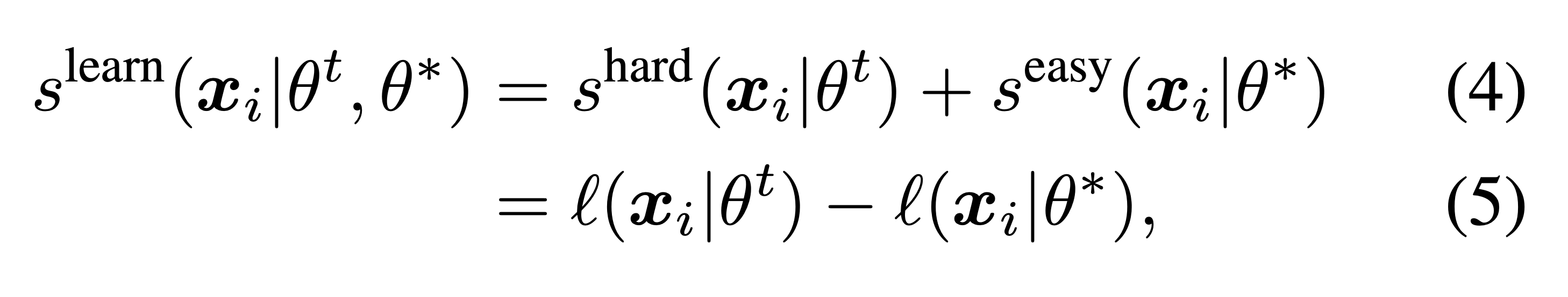
with the score defining an example as “learnable” if the model being trained has high loss for the example and a pretrained reference model has low loss.

When accounting for the cost of training and inference for the reference model, current approaches aren’t able to offer a net reduction in training costs.

Their method

The authors propose using a small model alongside the large model, and maintaining two sets of weights for the small model: pretrained reference weights $\theta_r$ and online “co-trained” weights $\theta_o$. The learnability score calculated cheaply with these two sets of weights on the full batch is used to select a subset of the batch for training the larger learner model $\theta_l$.

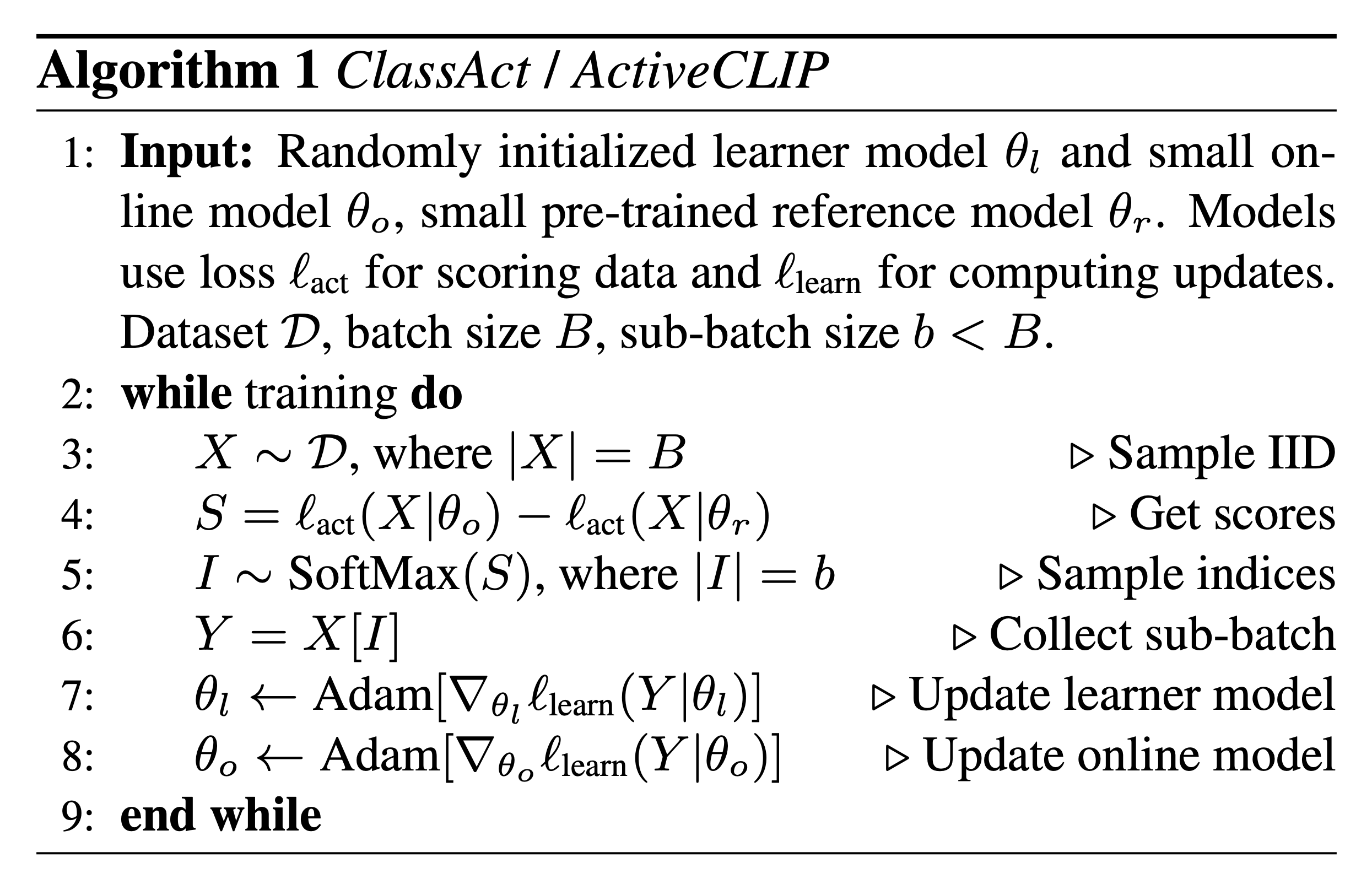
At this point a trade-off emerges. A larger scoring model is more effective at eliminating low-quality examples, but introduces greater overheads to training.

By balancing this trade-off, significant reductions in the overall training cost are possible.

Results

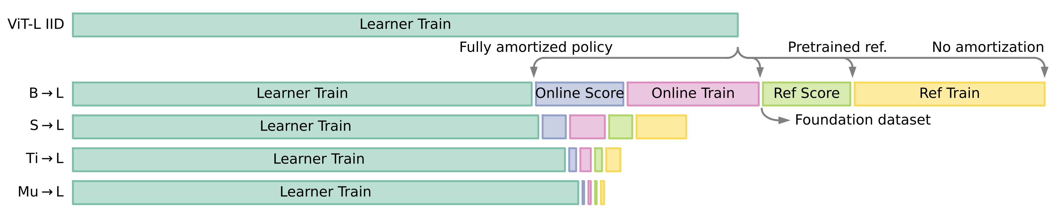
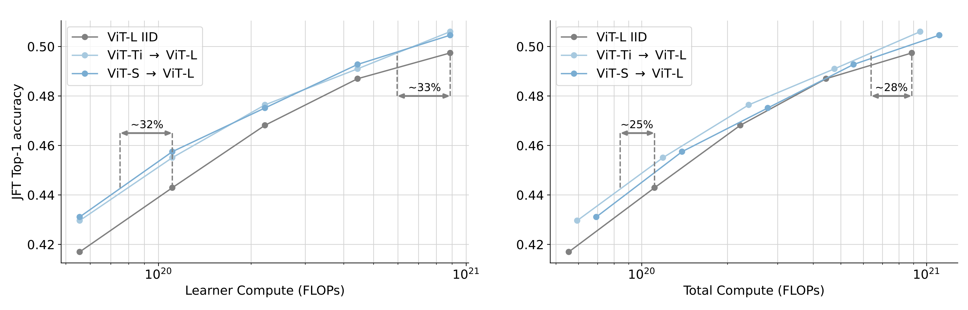
Their experiments are benchmarked against training ViT-L (304M params) on JFT (300M labeled images) for image classification or ViT-B (86M params) on the ALIGN dataset (1.8B image-text pairs) for multimodal image-text alignment.

With ViT-Tiny (5.6M params) as their reference model, they manage to obtain a consistent 25% reduction in training FLOPs to achieve the same downstream task accuracy when pre-trained on JFT ahead of time.

For image-text alignment, where large-scale datasets are typically much noisier, they manage to obtain 48% speedup (not clear if this is total FLOPs or training iterations) to target zero-shot accuracy on Imagenet-1k when pre-training their reference model on a smaller, cleaner multimodal dataset.

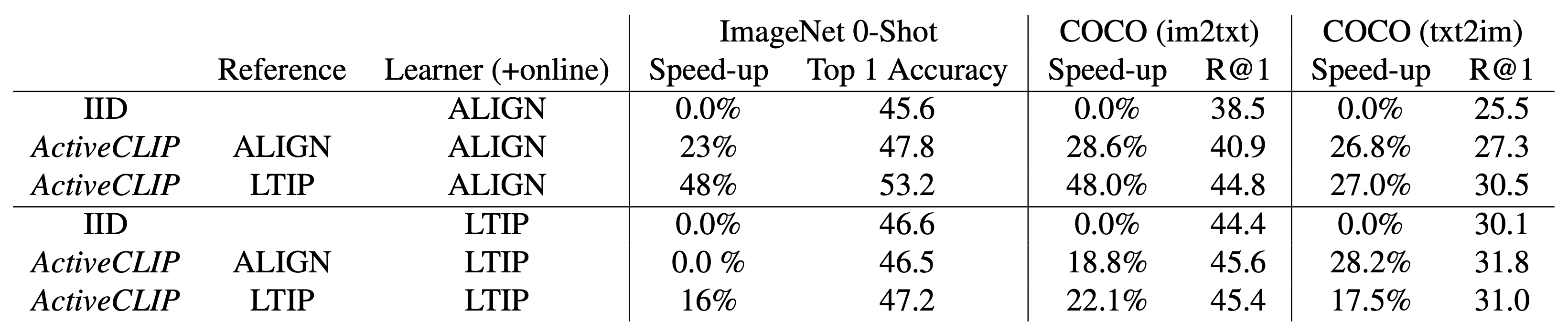
Impressive! Although, their numbers for zero-shot accuracy on ImageNet look a bit low for ViT-B trained on a 1.8B dataset (compare with OpenCLIP).

Takeaways

The FLOP reductions are encouraging. The technique is worth considering when training even larger models on larger, noisier web-scale datasets. It remains to be seen how difficult it will be to realise these FLOP or iteration reductions as wall-clock speed-ups, especially when needing to configure a cluster to support this kind of multi-scale workloads.