Analyzing and Improving the Training Dynamics of Diffusion Models

The key idea

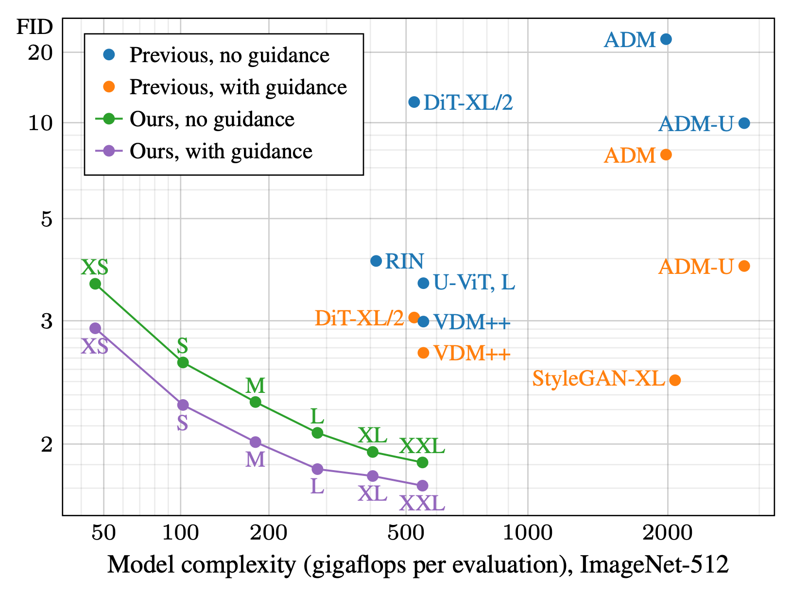
The architecture of diffusion models should be modified to ensure training signals are stable and predictable. This leads to a significant improvement in the quality of generated images.

The paper also introduces a second innovation: post-hoc EMA. To get the best final diffusion model it’s typical to take the exponential-moving-average (EMA) of the weights of the model throughout training. This “EMA version” of the model is usually something you build up during training, giving you one chance to get the right exponential weighting. The authors introduce a neat trick to re-construct any desired EMA weighting after training.

Their method

Training large diffusion models is often challenging due to inherently noisy training signals. The authors set out the following criteria to address this:

To learn efficiently in such a noisy training environment, the network should ideally have a predictable and even response to parameter updates.

Almost all current ML models fail to satisfy this. The paper suggests that this limits the performance of some models because of complex interactions between training dynamics and hyperparameters / architecture.

To address this, they modify their network to ensure constant magnitudes of activations, weights and updates in expectation. This is almost identical to the objective set out in Graphcore Research’s own unit scaling paper. A key difference here is that whereas unit scaling only satisfies this criterion at the beginning of training, they aim to maintain it more strictly throughout.

Their implementation proceeds through a series of steps (or “configs”) which they test / ablate at each stage. This is a great feature of the paper — we can see how useful each change is, justifying the many different tweaks they introduce.

Results

Their results for each config are as follows:

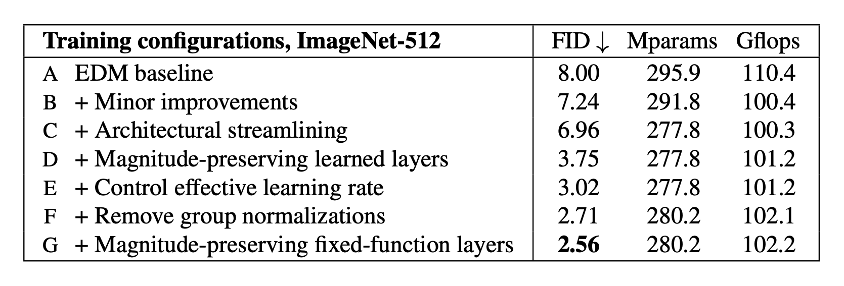
A few details of these configs are worth highlighting. Config D preserves activation magnitudes by dividing weights by their norm in the forward pass. Because of this, the initialisation-scale of the weights doesn’t matter and they can get away with using unit-initialisation.

They take this a step further in config E by permanently normalising the weights at every update. Interestingly, to ensure stable weight updates they still recommend normalising the weights a second time in the forward pass, due to the effect this has on the direction of the gradients. Combining all these tricks ensures a unified “effective learning rate” at all points in training, leading to substantial improvements.

In addition, their exponential-moving-average (EMA) trick also makes a big difference to the final performance. Their method works by taking intermediate moving-averages and linearly combining them after training, to approximate arbitrary-weight schedules:

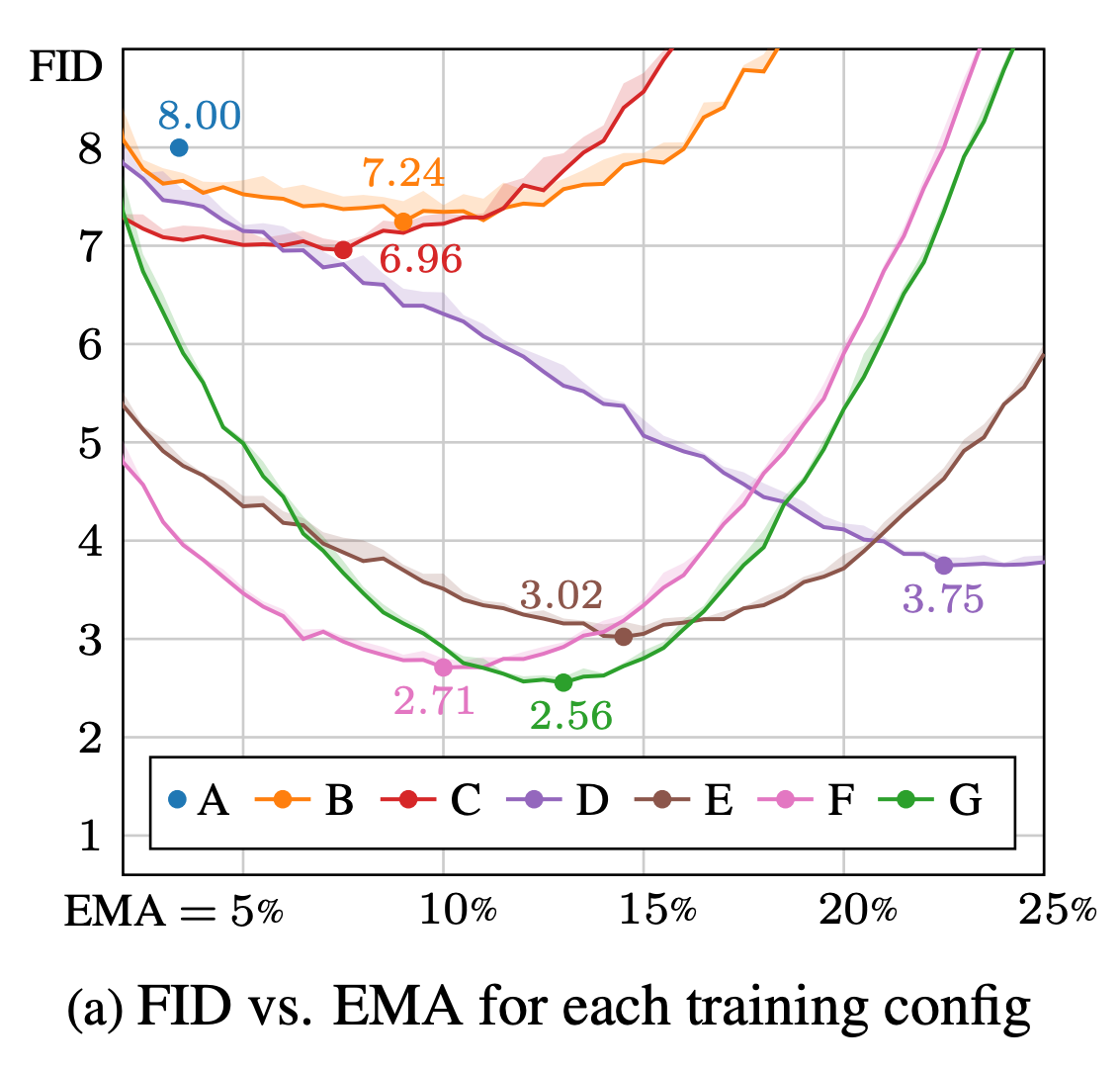
It’s clear that getting the schedule just right is important, and also hard to predict ahead of time. Until now the only option has been an expensive sweep, doing full training runs with different weightings. This innovation now makes the job of constructing the EMA substantially cheaper and easier — a big win for the community.