The Road Less Scheduled

The key idea

Deep learning practitioners use often use two key hacks to make optimisation of deep neural networks work in practice:

1. Learning rate schedules
2. Weight averaging for evaluation.

Here the authors propose a principled approach that replaces estimates of first-order gradient moments with an averaged parameter state to adapt commonly used optimisers to avoid the need for either of these hacks with no overhead.

Their method

We’ll present scheduled and schedule-free AdamW side-by-side, identify key differences, and explain how they are motivated.

Algorithm comparison

Given:

• initial parameter state $x_1$,
• learning rate $\gamma$,
• weight decay $\lambda$,
• warmup steps $T_{warmup}$,
• AdamW hyperparameters ($\beta_1$, $\beta_2$, $\epsilon$)

We compute:

Scheduled AdamW	Schedule-Free AdamW
Init $z_0 = 0$, $v_0 = 0$	Init $z_1 = x_1$, $v_0 = 0$
$\texttt{for t = 1 to T do}$	$\texttt{for t = 1 to T do}$
1: $g_t = \nabla f(x_t)$	1: $y_t = (1 - \beta_1)z_t + \beta_1x_t$
2: $z_t = (1 - \beta_1)z_{t-1} + \beta_1g_t$	2: $g_t = \nabla f(y_t)$
3: $v_t = (1 - \beta_2) v_{t-1} + \beta_2g_t^2$	3: $v_t = (1 - \beta_2) v_{t-1} + \beta_2g_t^2$
4: $\hat{z}_t = z_t/(1 - \beta_1^t)$, $\hat{v}_t = v_t/(1 - \beta_2^t)$	4: $\hat{v}_t = v_t/(1 - \beta_2^t)$
5: $\gamma_t = \gamma \textrm{min}(1, t/T_{warmup})$	5: $\gamma_t = \gamma \textrm{min}(1, t/T_{warmup})$
6:	6: $z_{t+1} = z_t - \gamma_t g_t/(\sqrt{\hat{v}_t} + \epsilon) - \gamma_t \lambda y_t$
7: $\alpha_t = \textrm{schedule}(t)$	7: $c_{t+1} = \gamma_t^2 / \sum^t_{i=1}{\gamma_i^2}$
8: $x_{t+1} = (1 - \alpha_t \gamma_t \lambda)x_t - \gamma_t\alpha_t \hat{z}_t/(\sqrt{\hat{v}_t} + \epsilon)$	8: $x_{t+1} = (1 - c_{t+1})x_t + c_{t+1}z_{t+1}$

Let’s go through line by line:

• Initialisation: Standard scheduled AdamW initialises gradient moment variables $z$ and $v$ at $0$. Schedule-free AdamW stores the second gradient moment variable $v$, and $z$ now represents a raw un-averaged parameter state, and is initialised to be the same as an averaged parameter state $x_t$
• Optimizer state updates (Lines 1-4): Standard scheduled AdamW computes gradients given current parameter state $x_t$ (Line 1) and update moments as an exponential moving average with temperatures $\beta_1$ and $\beta_2$ (Lines 2-3), and correct moment estimation bias (Line 4). Schedule-free AdamW first computes an interpolation $y_t$ between the raw $z_t$ and averaged $x_t$ parameter state (Line 1). We then compute gradients at this interpolated point (Line 2) and update the second moment (Line 3), and correct moment estimation bias (Line 4).
• Parameter state updates (Lines 5-8): Scheduled AdamW first determines learning rate coefficients given warmup and decay schedule (Lines 5-7), before applying the standard update rule using moments $z_t$, $v_t$ with weight decayed from $x_t$ (Line 8). Schedule-free AdamW likewise applies a warmup to the learning rate (Line 5), then updates the non-averaged parameter state $z_t$ using gradient estimate $g_t$, second moment $v_t$, and decays from interpolated weights $y_t$ (Line 6). We then update our weighted average of parameters $x_t$ with weights computed to discount parameters during warmup (Lines 7-8).

What motivates these changes?

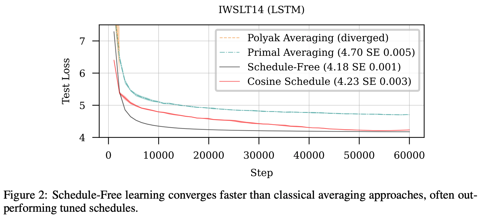
Previous work by the same group illustrated a connection between learning rate schedules and Polyak-Ruppert parameter averaging, a theoretically optimal technique for ensuring convergence in stochastic optimisation. Polyak-Ruppert parameter averaging is simple to compute (effectively just line 6-8 of our schedule-free algorithm), but appears to perform worse than cosine decay schedules in practice.

The authors propose combining Polyak-Ruppert averaging with Primal averaging. In Primal averaging, we evaluate gradients at a slow moving average parameter value rather than a fast moving immediate parameter value (standard practice). Likewise, Primal averaging on its own also appears to perform worse in practice as parameters change too slowly.

The combined solution is to effectively try to get the Primal average parameters to move a bit faster, by interpolating them with a Polyak-Ruppert average. This interpolated parameter is our $y_t$ term computed on Line 1. Given that when $\beta_1=1$ is pure Primal averaging, and $\beta_1=0$ is pure Polyak-Ruppert averaging, the authors’ recommended $\beta_1=0.9$ is still pretty close to Primal averaging.

Two other changes appear to be less theoretically motivated: using $y_t$ for decaying weights (rather than $x_t$ or $z_t$), and Polyak-Ruppert averaging coefficients $c_t$ that discounts parameter states visited during learning rate warmup. Warmup-free optimisers are a step too far it seems…

Results

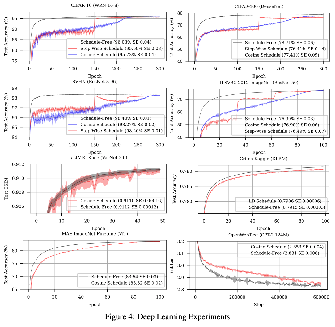
The authors test schedule-free optimiser on a battery of different small models of different types (Transformers, RNNs, CNNs, GNNs, Recommenders), different datasets and objective functions, In each case they show comparable convergence as carefully tuned learning rate schedules, with faster training dynamics in many cases.

Takeaways

As hacks go, learning rate schedules are an enduring one. Given the drastic effect they can have on your model performance when implemented in a training pipeline you omit them at your peril. However, they never seemed particularly well motivated other than for their empirical effect. This looks like a step in the right direction for hack-free optimisation in deep learning.